Anomalies can indicate that something’s about to go wrong in your environment. If you have a set of points, you can define which points are normal and which should be identified as abnormal. For example, points that cross a certain threshold might create an anomaly. To learn more about anomaly detection, see the blog Why is Operational Anomaly Detection So Hard?.
Functions for Anomaly Detection
You can use simple functions, prediction-based functions, or statistical functions to examine trends that might indicate an anomaly.
- Simple functions can give insight into the rate of change and trends.
- Prediction-based functions can help you compare actual values against expected values based on past performance.
- Statistical functions that return the mean, median, range, standard deviation, and inter-quartile range are great for understanding trends and variability in your data set. You can decide how much variability is normal. When datasets cross a certain threshold, they are detected as an anomaly.
Detect Anomalies with Simple Functions
A great way to do dynamic anomaly detection is a query like the following:
${data} / lag(10m,${data})
The result shows a 10-minute range of change as a ratio. You can change the time period to 1d or 30m to get the information you need.
This query calculates a rate of change between the current data and data from the series’ past performance. This results in a ratio of the current metric against the past data. This ratio helps you detect short-term changes, day-by-day changes, or even week-by-week changes.
Detect Anomalies with anomalous()
You can use the anomalous() prediction-based function to return the percentage of data points that have anomalous (unexpected) values. The function considers values considered anomalous if they fall outside a range of expected values. This range is centered around predictions based on past values. You can widen or narrow the range of expectation, typically to a number of standard deviations around the predictions.
For example, the following query considers points to be anomalous if they fall outside 95% of the expected values, or 2 standard deviations from the predictions:
anomalous(5m, .95, ts(my.metric))
Detect Anomalies with Mean and Median
The avg/ mavg and percentile/mmedian functions can help you understand the tendency of the data.
- Mean: Use
avgormavgto get the mean (average), that is, the number found in the middle of a set of values. The mean is affected and fluctuates easily even with single outlier.
*Median: Use the percentile() function to get the median, that is, percentile(50,<expression>[,<args]), or mmedian() to get the moving median. The median functions are more robust in dealing with outliers than avg/mavg because outliers tend to move the mean towards the outlier value.
Example: mavg() and mmedian()
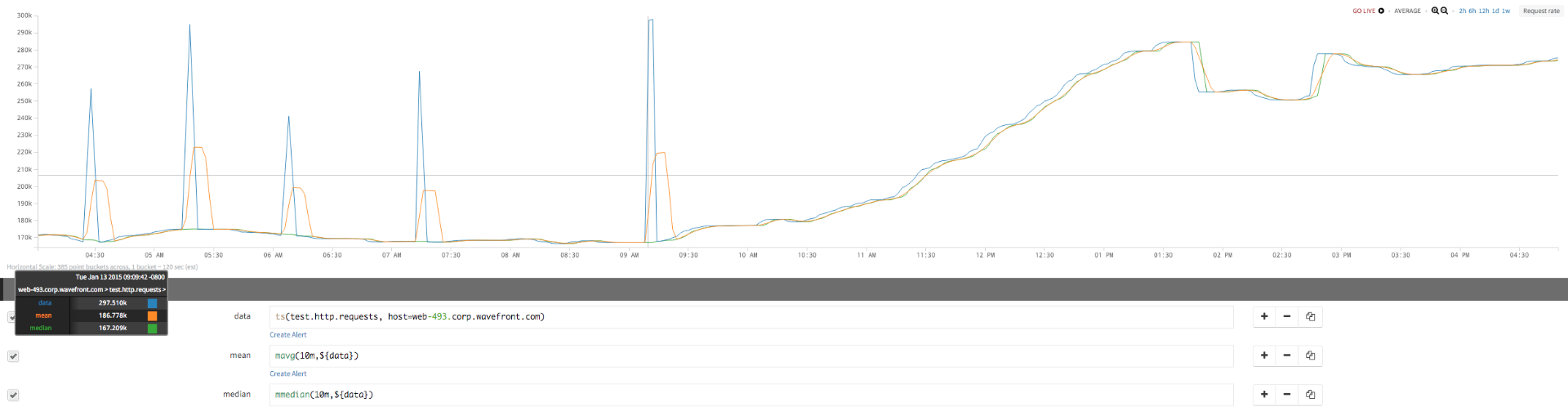
Consider the following queries that examine how mavg and mmedian behave in case of sudden spikes in the HTTP requests hitting a particular host:
| data: | ts(test.http.requests, host=web493.corp.example.com) |
| mean: | mavg(10m,${data}) |
| median: | mmedian(10m,${data}) |
The screen shot below shows the corresponding chart:
- If you consider these spikes as anomalies, use
avgormavgto catch similar deviations or variability. - If you consider the spikes as noise and want to ignore one-off spikes, use
percentileormmedian, which are less sensitive to outliers or variations, and show only sustained dips.
Detect Anomalies by Analyzing Data Spread
While the avg/ mavg and percentile/mmedian functions can help you understand the tendency of the data, Std Dev and IQR measure the spread of the data. If you want to use a level of dispersion or spread of the data as a function to define normal, you can use these functions to catch anomalies.
Standard deviation and IQR react to outliers (and to skewed data to some extent) in a similar way as mean and median respectively. Both help you understand the spread of the data over a range, but Std Dev is more sensitive to outliers and skewed data, while IQR is less sensitive.
Detect Anomalies with Standard Deviation
Standard deviation works well for detecting anomalies in data that is normally distributed. For uses cases like student grades in a class or the annual income across a set of population, which most likely has a normal distribution and tends to create a bell curve distribution, standard deviation can help you detect outliers, which are most likely on the either end of the curve.
- Tightly packed data – data whose values don’t vary over a wide range – have a low standard deviation value (closer to 0).
- A data set whose values are spread across a wide range has a high standard deviation.
Inter-Quartile Range
The inter-quartile range (IQR) indicates the extent to which the central 50% of values within the dataset are dispersed. IQR is based on, and related to, the median. In the same way that the median divides a dataset into two halves, it can be further divided into quarters by identifying the upper and lower quartiles. The lower quartile is found one quarter of the way along a dataset when the values have been arranged in order of magnitude; the upper quartile is found three quarters along the dataset. The inter-quartile range provides a clearer picture of the overall dataset by removing or ignoring the outlying values.
What function you use depends on your use case. Decide which statistical function works most effectively to define the normal behavior of your system and then use that function to detect anomalies.
Here are some examples for both Std Dev and IQR that illustrate these functions. See the reference page for anomalous for an example for that function.
Standard Deviation Example 1
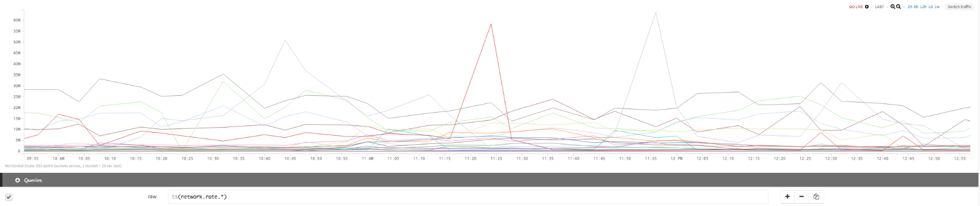
The following example first uses a query without standard deviation:
| raw: | ts(network.rate.*) |
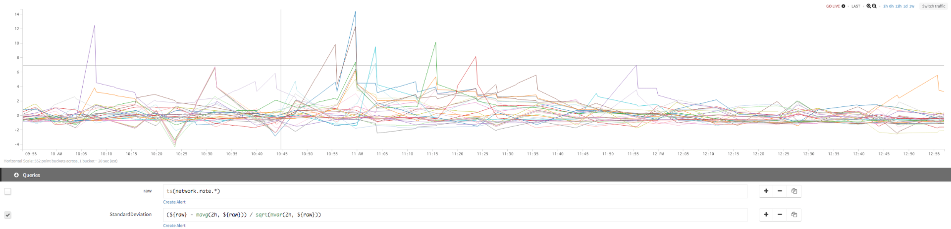
Then we add a query that builds on raw to get the standard deviation for the network rate:
| StandardDeviation: | (${raw} - mavg(2h, ${raw})) / sqrt(mvar(2h, {raw})) |
We use standard deviation to identify which series deviate greatly from their usual behavior, with a 2-hour moving window. When the standard deviation crosses a certain value (10 in this case), we have an anomaly. The same function is applied to different, widely scaled time series (each shown in a different color) and it identifies the spread of each series independently.
Query Without Standard Deviation
Adding Query With Standard Deviation
Standard Deviation Example 2
If the data is always distributed asymmetrically or is skewed, and you want to find anomalies in this skewed data, standard deviation does not work well, and you can try IQR.
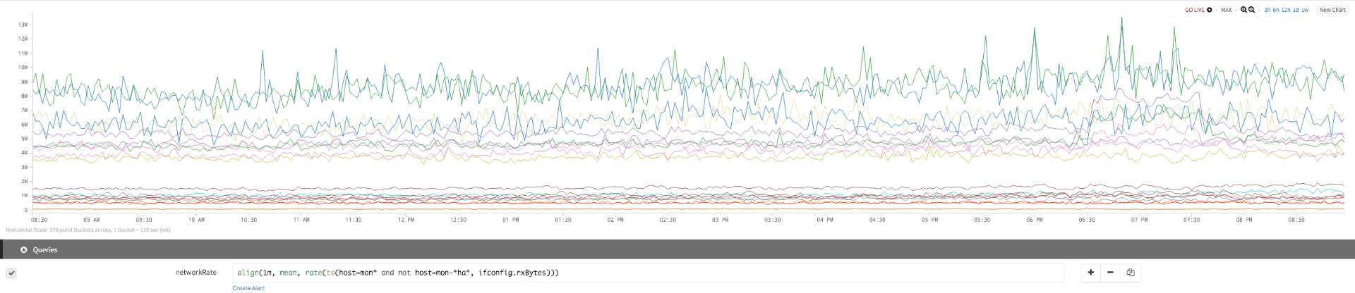
The time series in this example has a lot of spikes and troughs and we want to find a sustained spike in these seemingly noisy signals.
As you can see, standard deviation shows you the initial spike but starts decaying immediately. But if you use IQR, which has more resistance to the spikes and outliers, we see a sustained increase, making it easy to spot real outliers.
Data
The first chart uses the following query:
| network rate: | align(1m, mean, rate(ts(host=don* and not host=don-*ha*, ifconfig.rxBytes))) |
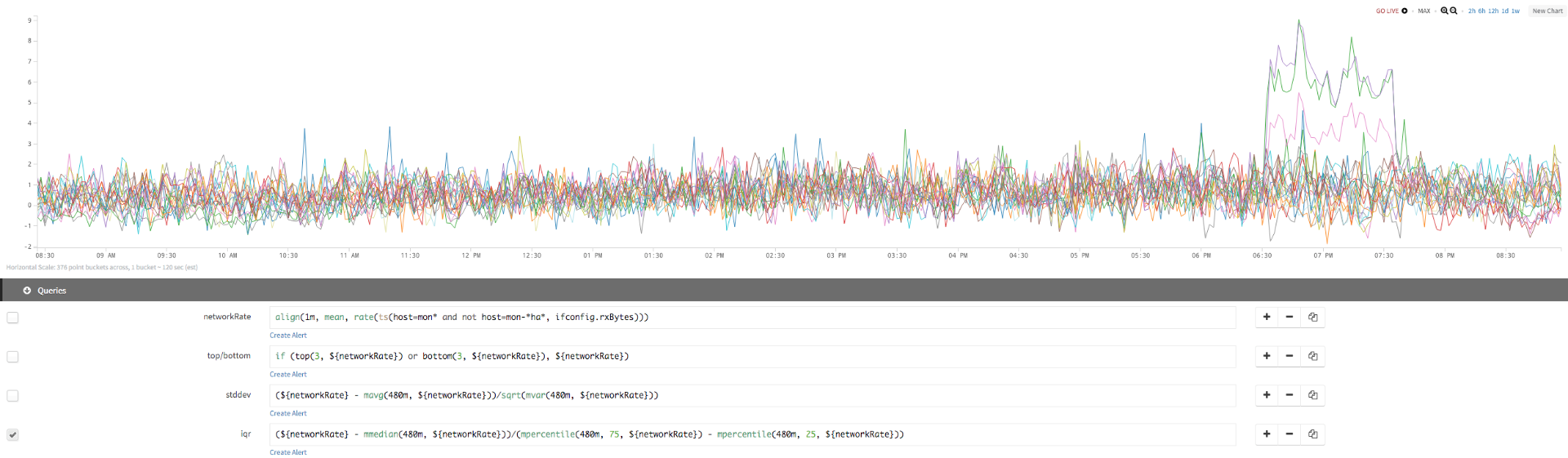
Std Dev
In the second chart, we add queries to see the standard deviation:
| network rate: | align(1m, mean, rate(ts(host=don* and not host=don-*ha*, ifconfig.rxBytes))) |
| top/bottom: | if (top(3, ${networkRate}) or bottom(3, ${networkRate}), ${networkRate}) |
| Std Dev: | (${networkRate} - mavg(480m, ${networkRate}))/sqrt(mvar(480m, ${networkRate})) |
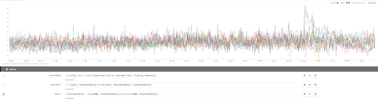
IQR But we see the information we’re after only when we add the IQR query:
| network rate | align(1m, mean, rate(ts(host=don* and not host=don-*ha*, ifconfig.rxBytes))) |
| top/bottom | if (top(3, ${networkRate}) or bottom(3, ${networkRate}), ${networkRate}) |
| Std Dev | (${networkRate} - mavg(480m, ${networkRate}))/sqrt(mvar(480m, ${networkRate})) |
| IQR | (${networkRate} - mmedian (480m, ${networkRate}))/(mpercentile(480m, 75, ${networkRate}) - mpercentile(480m, 25, ${networkRate})) |
Standard Deviation Example 3
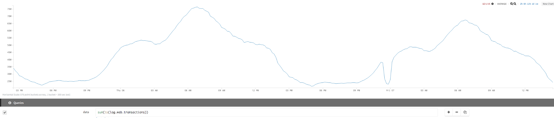
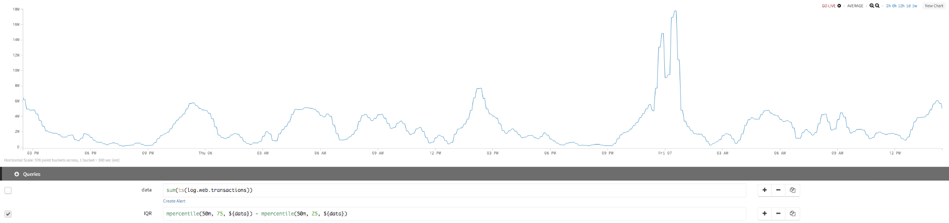
In this example, a time series deviates and continues oscillating over a day over range – this is the normal behavior of the series). When you try to spot an anomaly in the oscillating data using std dev in a 1h or 2h window, standard deviation does not really capture the dip as well as IQR because the distribution of data in a moving 2h window is not normal. If you look at IQR, you see that it also fluctuates in the moving 2h window, but not as much as std dev, and it spikes in case of an immediate dip in the oscillating signal.
Data
| initial query | sum(ts(log.web.transactions)) |
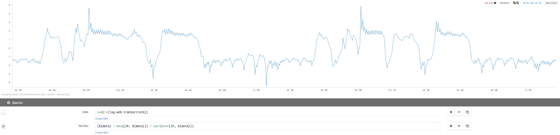
Std Dev We can add a second query to see the standard deviation:
| initial query | sum(ts(log.web.transactions)) |
| Std Dev | (${data} - mavg(1h, ${data})) / sqrt(mvar(1h, ${data})) |
IQR
IQR gives us more information about the time series:
| initial query | sum(ts(log.web.transactions)) |
| IQR | mpercentile (50m, 75, ${data}) - mpercentile (50m, 25, ${data}) |
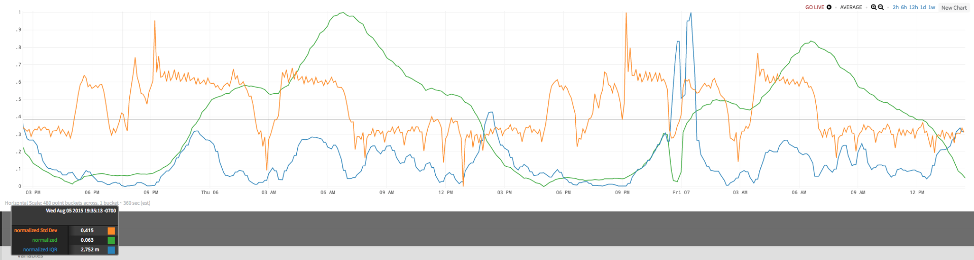
The chart below shows the normalized values for all three series. Looking at this chart, with values for the initial query, the standard deviation, and the IQR, illustrates how they differ.
Comparing Current Behavior to Past Behaviors
Comparing current behavior with past behavior requires determining a baseline from past behavior. The strategy (or combination of strategies) that works best depends on your use case.
Using the Previous Week as a Baseline
You can compare current behavior to last week’s behavior with the lag() function. Assume the query that specifies current behavior can be referenced with the query line variable ${current}. Then this query compares the current behavior with last week’s behavior:
${current}/lag(1w, ${current})
The query returns the ratio between current behavior and what it was a week ago. It’s easy to make this a percentage change instead of a ratio. Or, you could instead compare the current behavior with a different point in time, such as the previous day, instead of the previous week.
Using the Average Behavior of the Last X Weeks as a Baseline
You can also work with several weeks’ worth of behavior rather than just the previous week. For example, suppose you to establish a baseline using the last 3 weeks’ worth of behavior. You’d have 3 queries to specify the behavior for each of the previous 3 weeks:
1-week: ${current}/lag(1w, ${current})
2-week: ${current}/lag(2w, ${current})
3-week: ${current}/lag(3w, ${current})
You can find the average behavior from these 3 weeks with this query:
baseline: (${1-week}+${2-week}+${3-week})/3
or
baseline: rawavg(collect(${1-week},${2-week},${3-week}))
Again, you can determine a ratio of the current behavior against this baseline like this:
${current}/${baseline}
Instead of an average, you could calculate other statistics.